cos θ ∣0❭ + sin θ ∣1❭
And then with probability cos2 θ the observation will be "the photon passes through the filter" and the quantum state of the photon will be ∣0❭. Otherwise, necessarily with probability,
1 - cos2 θ = sin2 θ
the photon will be absorbed by the filter and photon would have quantum state ∣1❭.
In the case of θ = 45 degrees, the quantum state has the name ∣+❭ and the output of a stream of photons of this state passing through a polaroid filter with measurement basis ∣0❭, ∣1❭ would be a truly random and unbiased coin flip deciding whether the photon passes or is absorbed.
When a quantum state is written as a linear sum of quantum states at can be outcomes of a measurement, gives Born's Law for the probability that the measurement will achieve a particular outcome — it is the square of the coefficient that weighs that outcome in the linear sum expressing the quantum state.
If a superposed state is put as an input into a quantum computation, it is as if the component states of the superposition were being simultaneously and independently input into the computation. Hence, we have parallel computation that will flow through a single computation path. In the case of the superposed state ∣+❭, it will be as if the output on input ∣0❭ is being calculated at the same time and with the same hardware and memory registers as the output on input ∣1❭.
A superposed state is truly a quantum phenomenon. It is the famous Schrodinger's cat paradox, in which, if Schrodinger's cat is so isolated from any measurement or observation that it can be held in a quantum state, it could both dead and alive at the same time. Beware the moment any observation is made about the cat for then the cat must become some state that is permitted classically. It has to either become dead or become alive.
We will also do several other experiments in superposition, entanglement, and quantum algorithms, on quantum computers made available through the IBM Quantum Experience
If you wish, you can create an IBM Q account and explore on your own.
The IBM Quantum Experience has a convenient graphic front end running in a browser, for one's first contact with quantum computing. There is a more sophisticated interface using the qiskit library, a Python package. We will use Jupyter notebooks and qiskit to define quantum circuits, to transpile (compile) the circuits into the machine code of one of IBM's available quantum computers, and to submit the job to be run on the quantum compter (our simulated either locally using AER or remotely using IBM's more advanced simulators).
Once you have created your IBM account, you will receive an account token, the is loaded into a local configuration file using the qiskit library call to IBMQ.save_account. A provider is then provided to a Python session using IBMQ.load_account. The Provider object has various Backend objects, that have, for instance, run methods for submitting a quantum circuit description to the backend, such as a quantum computer, for running on the machine.
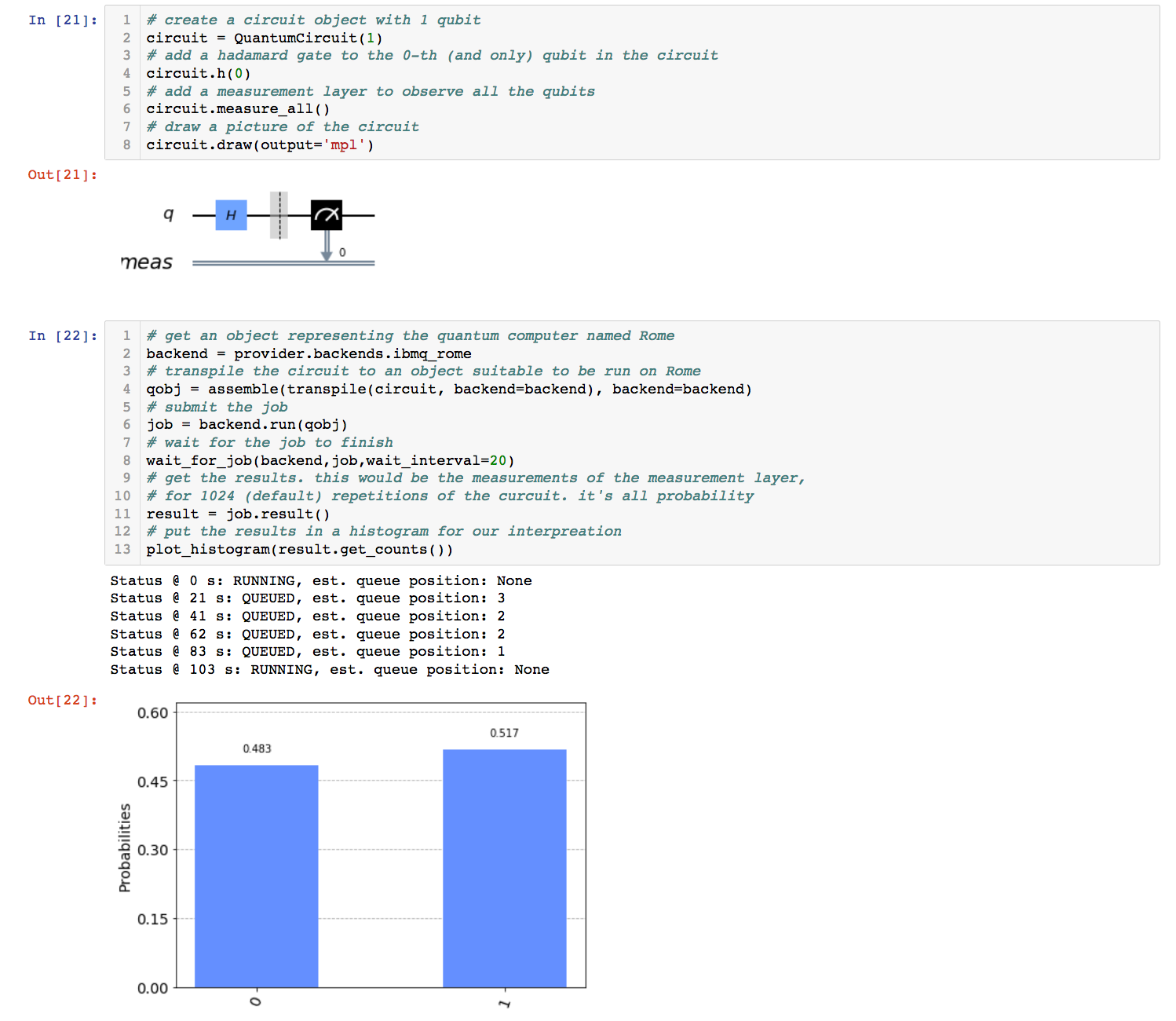
Here is sample Jupyter notebook code that runs our quantum coin flip on the IBM 5 qubit quantum computer named Rome. I give a table of contents of the code.
# Importing standard Qiskit libraries and configuring account
from qiskit import QuantumCircuit, execute, Aer, IBMQ
from qiskit.compiler import transpile, assemble
from qiskit.tools.jupyter import *
from qiskit.visualization import *
from qiskit.providers.jobstatus import JOB_FINAL_STATES, JobStatus
from qiskit import QuantumCircuit, QuantumRegister, ClassicalRegister, execute, Aer

import time

# Loading IBM Q account(s)
provider = IBMQ.load_account()


# a helper function

def wait_for_job(backend,job,wait_interval=5):
    retrieved_job = backend.retrieve_job(job.job_id())
    start_time = time.time()
    job_status = job.status()
    while job_status not in JOB_FINAL_STATES:
        print(f'Status @ {time.time()-start_time:0.0f} s: {job_status.name},'
              f' est. queue position: {job.queue_position()}')
        time.sleep(wait_interval)
        job_status = job.status()

# Define the Quantum and Classical Registers
q = QuantumRegister(1)
c = ClassicalRegister(1)

# Build the circuit
superposition_state = QuantumCircuit(q, c)
superposition_state.h(q)
superposition_state.measure(q, c)

# draw the circuit
draw_circuit = False
if draw_circuit:
    superposition_state.draw(output='mpl').savefig("myfile.png",dpi=150)

# Execute the circuit
backend = provider.backends.ibmq_rome
qobj = assemble(transpile(superposition_state, backend=backend), backend=backend)
job = backend.run(qobj)
retrieved_job = backend.retrieve_job(job.job_id())

# Wait for completetion
wait_for_job(backend,job)

result = job.result()
print(result.get_counts())

---------------

# ran on 28 april 2020
# program prints:


Status @ 1 s: RUNNING, est. queue position: None
Status @ 6 s: RUNNING, est. queue position: None
Status @ 11 s: RUNNING, est. queue position: None
{'1': 568, '0': 456}
The device that can set a qubit in a superposed state is called a Hadamard gate, named after the mathematican Jaques Hadamard, who proposed the linear transformation that achieves the superposition mathematically. In a quantum computer, if a hadamard gate H is applied to a quantum state ∣0❭ the result is the superposition of ∣0❭ and ∣1❭ scaled to unit length
∣+❭ = (1/√2) ∣0❭ + (1/√2) ∣1❭
If after the application of a hadamard gate, a measurement is taken in the ∣0❭, ∣1❭ basis, but Born's (1/√2)2 = 1/2 of the time the measurement is 0, and the other half it is 1.
As the choice will be truly random, our first circuit is then a random bit generator.
∣q1❭ ⊗ ∣q0❭ = ∣q1 q0❭
where ⊗ is the tensor product, and is how qubits are combined.
The following circuit creates the superposition, ∣00❭ + ∣01❭ + ∣10❭ + ∣11❭
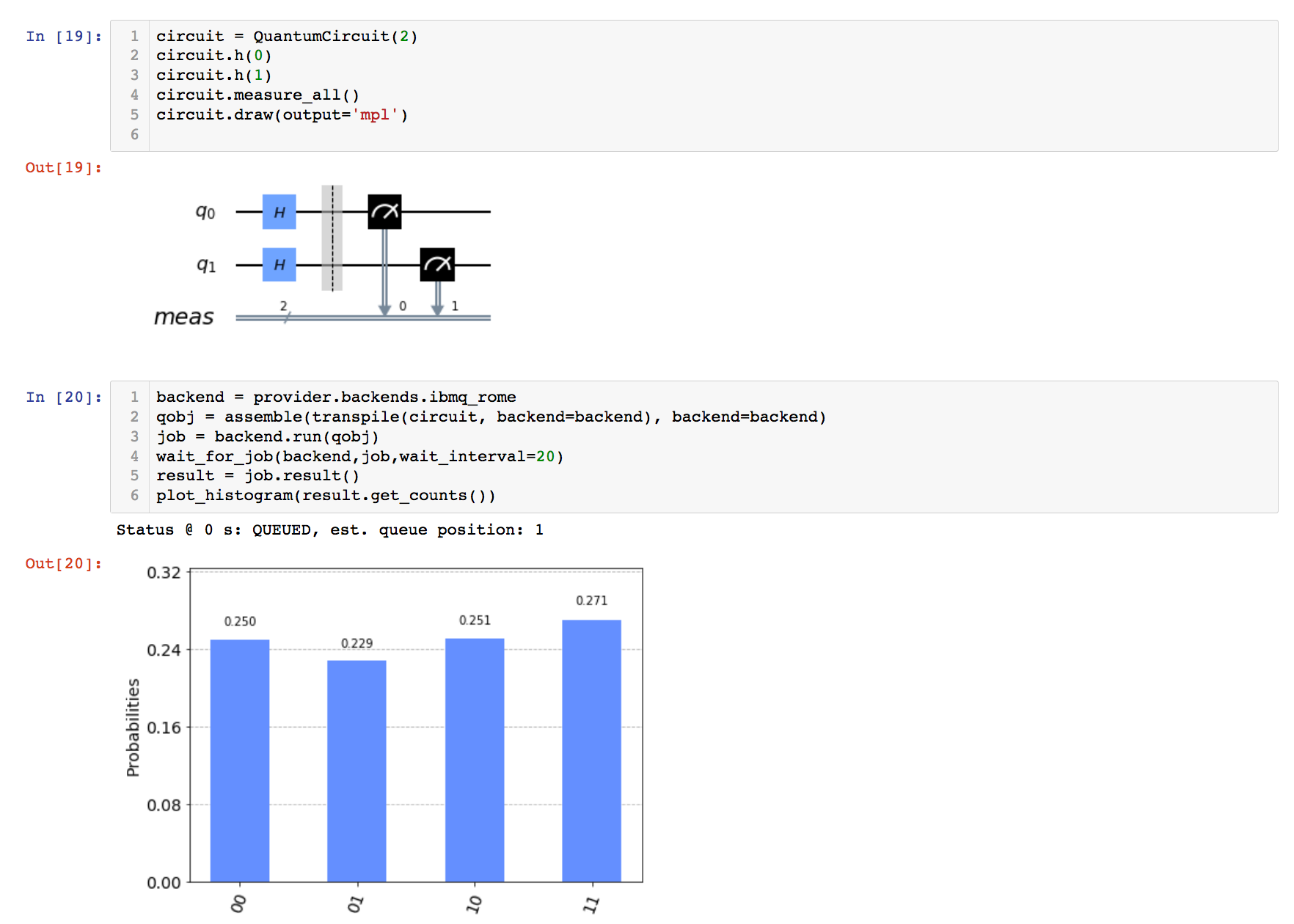
Note the result of a hadamard applied to any single qubit — it interacts with all the other qubits in a manner that forms all possible combinations. If you wish, you can get this from the distributive law. I will do a simplified example of two qubits,
H(∣0❭) ⊗ H(∣0❭)
=
∣+❭ ⊗ ∣+❭
= (1/√2) (∣0❭ + ∣1❭ )
⊗
(1/√2) (∣0❭ + ∣1❭ )
= (1/2) ( ∣0❭ ⊗ ∣0❭
+ ∣0❭ ⊗ ∣1❭
+ ∣1❭ ⊗ ∣0❭
+ ∣1❭ ⊗ ∣1❭
)
This is the action of the tensor product, denoted with symbol ⊗. In many ways its algebraic properties as the same as the common product, except that it is not commutative. That is, a ⊗ b ≠ b ⊗ a, in general. As with the product, the tensor product sign is often dropped, so ∣0❭ ∣0❭, ∣00❭ and ∣0❭ ⊗ ∣0❭ are all the same thing.
Note the equal weighting of 1/√2 on each state. Recalling Born's rule, a measurement will bring the quantum state to one of these four classical states with probability 1/4. Which is what happend on the quantum computer Rome, as shown in the box above.
For multiple qubits, to make things easier to read, a sequence of qubits, such as the three qubits ∣101❭ and be written by using the base 10 notation for the bit string. In this case, ∣5❭. Note that this notation is a bit deficient, since ∣5❭ could mean ∣101❭ or ∣0101❭ or ∣00101❭. One must look into the context of the discussion to decide which of these, or some other, is meant.

author: burton rosenberg
created: 28 apr 2020
update: 4 may 2020