This is rough draft of a resume of ideas of discrete probability. A work in progress.
Contents:
Probability is the mathematical theory of chance occurrences or other situations of uncertainty. It provides a framework for considering chance and uncertainty and a method to calculate likelihood of events. There are at least two different intuitive basis for probability: the Frequentist and the Partial Belief. The Partial Belief is aligned with what is called Bayesian Statistics, but the Frequentist model appears to be the most common and simplest.
The Frequentist would claim that the probability of a coin being tossed and landing heads is 1/2 because half the time the experiment of tossing a coin is attempted, the outcome is it lands heads. In this viewpoint, probability is an average occurrence over a number of repeated trials. This is the most common view of probability.
If one says there is a 50% probability of rain, however, this means something a bit different, since the day cannot be repeated a number of times, with about half the days raining and half not. In this usage probability models a belief in something happening. A coin coming up heads with probability 1/2 on some particular toss is another example. This is not a question of what the coin will do on average, but what it will do specifically on the next toss. A probability in this sense expresses the Partial Belief in an event occurring.
Either intuitive basis is supported by the formal model of probability. For continuous probability, this formalism is called Measure Theory. For the simpler finite case, it is simply a form of counting. It is an abstract mathematical approach to probability consisting of a set of outcomes, or states-of-the-world, a collection of events formed as sets of outcomes, and a measurement function which can be applied to events which satisfies a bunch of axioms, the Axioms of Probabilities.
The Law of Large Numbers is proved in the formal theory. It says that if the probability of an event is p (whatever that means), then in a series of repeated trials, a fraction p trials will result in the event happening. The Law of Large Numbers therefore allows the Frequentist to adopt the formal model. It can be used to assign meaning to probability according to the Frequentist's intuition.
The collection of events has a structure, and this structure can be exploited by the Partial Belief modelers to interpret probability according to their intuitions. The abstract theory of probability is a good basis for either interpretation, and is of itself fairly philosophy-free, so it is easy for calculations.
Probability models chance occurrences, or other situations of uncertainty. The philosophical underpinnings of chance and belief is complicated, but probability simplifies all issues into a set, called the probability space, subsets of the space, called events, and a measurement function from events to real numbers in the range 0 to 1, called the probability (or measure). The collection of events and the probability function must satisfy some formal properties, called the axioms of probability. As a piece of mathematics, probability theory is certainly true. However, if its correspondence to reality can only be judged empirically: does it give useful results? Can I use probability to play the odds and win.
Consider the throwing of a many-headed die. If the die has n sides, the throw can result in the showing of exactly one of the sides. This is called an outcome. (In the textbook, CLR, an outcome is called an elementary event.) Each outcome has a probability which is the likelihood of the outcome, expressed as a fraction from 0 to 1. If an outcome never occurs, it is impossible, its probability is 0. If the outcome always occur, it is certain, its probability is 1.
We refer to the throwing of the die as an experiment. Denote that the experiment X resulted in outcome x by the symbol X=x. It is usual that experiments are named with uppercase letters and outcomes with lower case letters. The probability that experiment X results in outcome x is denoted Prob(X=x).
Rule: Since one and exactly one of the outcomes must occur, the probabilities must sum to 1.
Prob(X=1) + Prob(X=2) + ... + Prob(X=n) = 1
Example: A coin is a 2-header die and we generally speak of heads H or tails T, rather than 1 or 2. The outcomes heads and tails are equally likely, so,
Prob(X=H) = Prob(X=T) = 1/2
The collection of all possible outcomes of an experiment is the probability space. In each experiment one and only one outcome occurs. A set of outcomes is called an event. The probability of an event is the sum of the probabilities of all outcomes in the event. It is the likelihood the an experiment will give an outcome that is in the event.
Example: We can list all the possible events of a coin toss. They are,
If F and G are events, then the intersection and union of these sets are also events. The intersection F ∩ G is the event that an experiment has outcome in both F and G; the union F ∪ G is the event that an experiment has outcome in either F or G.
Rule: If F and G are events with no common element, that is, no outcome is both F and G, then the probability of F ∪ G is the sum of the probabilities of F and G individually,
Prob( F ∪ G ) = Prob(F) + Prob(G) ( if F ∩ G = ∅ )If !E is the complement of event E, then Prob(!E ∪ E ) =1, because it is certain that E either happens or it doesn't. Since,
Prob( !E ∪ E ) = Prob(!E) + Prob(E) = 1,then,
Prob(E) = 1 - Prob(!E).
Example: Consider two dice. The probability space is all pairs of numbers (i,j), i and j a number 1 through 6. There are 36 different outcomes, (1,1), (1,2), ..., (6,6). Each is equally likely so,
Prob(X=(1,1)) = Prob(X=(1,2)) = ... = Prob((6,6)) = 1/36.A possible event is "a seven is rolled". This event is the set of outcomes,
E = {(1,6), (2,5), (3,4), (4,3), (5,2), (6,1)}.
The probability of the event is,
   Prob(E) = Prob({(1,6), (2,5), (3,4), (4,3), (5,2), (6,1)})
           = Prob(X=(1,6)) + Prob(X=(2,5)) + ... + Prob(X=(6,1))
           = 6/36 = 1/6.
Exercise: What is the event that two die role a even total? What is the probability of this event?
Experiment: Roll two dice 120 times and count the number of sevens. Is the count close to 20? How could I predict this? How come it was not exactly 20? How could I predict that it would not be exactly 20?
The collection of all events can get complicated. In discrete probability theory, each elementary event or outcome can be measured — each outcome has a value by the probability function. The general theory says that if events E and F can be measured so can E ∩ F, the event of simultaneously attaining events E and F; and so can the event E ∪ F, the event of either one or the other (or both) E or F attaining.
There is an additional requirement dealing with an infinite series of events. Of course, there are no essentially infinite series in finite probability.
For discrete probability these requirements on the class of event leads to the simple notation that an event is any subset of the entire probability space. However, continuous probability requires the statement about the collection subsets of the probability space that will be considered events. The interested reader will find it extremely fascinating to figure out what this means.
A probability event is a subset of the universe of possible outcomes for an experiment. To each event is attached a number between 0 and 1, the probability of the event. Events maybe connected so that knowledge whether one event has occurred allows a better prediction of the whether or not a second even has occurred. Events might overlap as subsets, and the more they overlap the more one event predicts another.
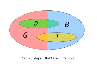
Example: Consider a collection of 20 children, 10 girls and 10 boys. The experiment is to choose one child at random. The space will be called X, the set of boys B and the set of girls G are both subsets of X. They are events. We can ask having chosen a child whether that child is a boy or a girl, equivalently, whether the outcome x from X is an element of the set B or the set G.
If the choice is made randomly, which here means with a uniform and equal likelihood of any child being drawn, then the probability of the event a boy is drawn is equal that a girl is drawn, both being 1/2. Prob(B)=Prob(G)=1/2.
The boys and girls show a preference for one of two toys, dolls and trucks. The set of children who prefer dolls is D, and those that prefer trucks is T. As with B and G, D and T will neatly divide the set of C into two subsets which together contain all children without overlap.
I will assume that girls show a tendency to prefer dolls, and boys trucks. To make the numbers easy to follow, assume among the 10 girls, 8 prefer dolls, and 2 prefer trucks, and among the 10 boys, 2 prefer dolls and 8 prefer trucks. In symbols:
I have tried to draw a picture of the situation. The large circle encloses elements (not drawn), one element for each child. The circle is divided equally and labeled G and B, indicating that half of the enclosed elements are of the set G, girls, and half of the set B, boys. Two additional circles are drawn, on to enclose D, the set of children preferring dolls, and the other to enclose T, the set of children preferring trains. The circles are drawn to overlap B and G roughly in proportion to the number of children of each gender liking each toy.
From this data we already know the probability of a child chosen randomly of preferring dolls, it is the probability of the experiment yielding a child in the set D, or 1/2. Likewise for a random child preferring trucks. But if we knew that the child chosen was a girl, it becomes more likely that the child prefers a doll, given this knowledge. We are asking for the conditional probability that an c drawn from C, given that c is in G, then c is in D. This is the conditional probability of D given G, and is written Prob(D|G). It should be intuitively clear that Prob(D|G)=4/5, since if we limit our considerations to just girls, 8 out of 10 prefer dolls.
There is a formula for conditional probability which supports this result:
Prob(D|G) = Prob(D ∩ G)/Prob(G)
In this case, Prob(D ∩ G)=8/20=2/5 and Prob(G) = 10/20 = 1/2.
For this formula to work, Prob(G) must not be zero. For discrete probability,
this means that you cannot condition on an impossibility. It has no meaning.
(For continuous probability, however, events may have probability
zero without being impossible, and calculus is needed to sum over these
infinitesimals to get a finite number.)
A similar question is this: given a child picked at random, the probability that the child is a girl is 1/2. Given the additional information that the child prefers dolls, the probability of the child being a girl rises to 4/5. This is the conditional probably of the event G given the event D, Prob(G|D), and the calculation is:
Prob(G|D) = Prob(G ∩ D)/Prob(D) = (8/20) / (10/20) = 4/5
Given two events F and G, the probability of event G might depend on whether F has also occurred. For instance, the probability of a die being six is related to the probability that the die rolls and even. Given that a six has been rolled, it is then certain that an even number has been rolled. Given that an even has been rolled, it is now more likely that a six has been rolled.
From the definition of conditional probability, there is this definition for the probability of the conjunct of events:
Prob(D ∩ G) = Prob(D|G) Prob(G)
This is more general that the definition for independent D and G
(see below), and effectively "explains" the impact of non-independence
on the formula.
Intuitively, independence of two events is that the likelihood of one event is not changed by the occurrence of the other event. We learn nothing about the first having observed the second. So,
Prob(F|G) = Prob(F).Using the definition,
Prob(F|G) = Prob(F ∩ G)/Prob(G)
we have that F and G are independent exactly when,
Prob(F ∩ G) = Prob(F) Prob(G) *Definition*This is the definition for independence. It is also an important rule for the calculation of the probability of a joint event given the probabilities of the component events, in the case where the events are independent.
Working probabilities with independent events is much easier than with dependent events because of this rule.
The definition of Independence is philosophically taxing. Intuitively, it should be that F and G are independent if there is no causal connection between them, and dependent otherwise. In this view, dependence of events has a deeper meaning: the presence of a mechanism by which the events affect each other. This may be the scientific understanding, but it is not the mathematical understanding. The mathematical understanding is about predictability, not causality. Even if there is a causal connection between F and G, they are mathematically independent if this connection doesn't change the predictability of one event by the other. Conversely, if observation of one event biases the probability of another event, they are dependent, and it is not necessary to wonder about whatever mechanism causes the dependence.
Example: What is the probability that two die roll a total of 9 given that the first die rolls a 6? Are the events "first die is a 6" and "total is 9" dependent or independent?
The event E = "total is 9" contains {(3,6), (4,5), (5,4), (6,3)}. So,
Prob(E) = 4/36 = 1/9.Let F be the event "first die rolls a 6". F contains 6 events,
{(6,1), (6,2), ..., (6,6)}.
Hence Prob(F)=6/36=1/6. Also E ∩ F={(6,3)} and Prob(E ∩ F)=1/36.
So,
Prob(E|F) = Prob(E ∩ F)/Prob(F) = (1/36)/(1/6) = 1/6.Since Prob(E)<Prof(E|F) the events are dependent. It is more likely to have a total of 9 if it becomes known that the first die rolled a 6. (Intuitively, cases have been excluded where the first die rolls a value for which a total of 9 is impossible, such as the first dice being a 2.)
Exercise: What is the probability that the second of two die rolls a 3 given that the first rolls a 6. Are the events "first die is a 6" and "second die is a 4" dependent or independent?
Example: What is the probability that two die roll an even total given that the first die rolls a 6? Are the events "first die is a 6" and "total is even" dependent or independent? Does the sum "depend" upon the value of the first die?
Call F the event the first die rolls a 6, and G that the total is even. Of 36 possible rolls of both die, 6 are events in F. So Prob(F)=6/26=1/6. There a three ways, each equally likely, that the total is even and the first roll is a six. So Prob(F∩G)=3/36=1/12.
Prob(G|F) = Prob(F ∩ G)/Prob(F) = (1/12)/(1/6) = 1/2The Prob(G) is the number of ways to roll an even divided by the 36 different possible rolls. Doing the counting, we have Prob(G)=1/2. So Prob(G|F)=Prob(G).
The events F and G are independent, even though the total does certainly "depend" on the outcome of the first roll.
If there is a dependence between two events, F and G, it is often easier to calculate the probability of F assuming G than the probability of G or of F ∩ G. In that case, the law of conditional probability can be used in this form,
Prob(G|F) Prob (F) = Prob( F ∩ G )
I really owe you all an example of this.
Exercise: Suggest a good example of using the above formula of a way to calculate Prob( F ∩ G ) when F and G are dependent, and direction calculation of Prob( F ∩ G ) is confusing.
By the definition of conditional independence, P(H and G)/P(G), if H and G are independent, in the sense P(G|H)=P(G), then P(H and G)=P(H)P(G), and therefore
P(H|G) = P(H ∩ G)/P(G) = P(H)P(G)/P(G) = P(H).
So if truck/doll-favoritism does not predict gender, it follows that
gender does not predict truck/doll-favoritism. It's an interesting
mathematical fact to keep in mind.
In summary, their are three equivalent definitions of independence:
   ** Definitions of independence of events G and H **

   (1) P(G|H) = P(G)
   (2) P(H|G) = P(H)
   (3) P(G ∩ H) = P(G)P(H)
Bayes Law allows for the calculation of conditional probabilities when interchanging which event is the given event.
Prob(F|G) = Prob(G|F) Prob(F) / Prob(G)
The probability of F given G is related to the probability of G given F
by the ratio of the probabilities of F and G.
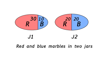
For example, suppose there are two jars, each with 40 red and blue marbles. Jar one, J1 has 30 red and 10 blue marbles. Jar two, J2 has 20 red and 20 blue marbles. A marble is chosen at random by first choosing between jar one and jar two at random, each equally likely, and then drawing a marble out of the chosen jar at random. Therefore each marble is equally likely to be drawn.
However, if jar one is chosen, a red marble is more likely. And conversely, if the result of the random draw, then it is more likely that jar one was chosen in the first step of the draw. Bayes gives a way of calculating exactly how likely. By the definition of conditional probability, the probability of the event (J1 and Red) can be expressed in two ways:
Prob(J1 and Red) = Prob(J1|Red) Prob(Red)and
Prob(J1 and Red) = Prob(Red|J1) Prob(J1)
Prob(J1|Red) = Prob(Red|J1) Prob(J1) / Prob(Red)The point is Prob(Red|J1) is easy to calculate: 30/40. And so is Prob(Red) = 50/80, and Prob(J1) = 1/2. So:
Prob(J1|Red) = (30/40) (1/2) / (50/80) = 3/5.Given that a red marble was chosen, it is 3 out of 5 likely that you had drawn from jar one.
Often what is observed from an experiment is not the outcome but some measurement of the outcome. A random person's height is the measurement (height) of a randomly drawn person. The average or typical height of a person is a fact about the measurement. A random variable is a function that attaches a value to an outcome, such as the height of a randomly chosen person. A random variable can be used to create events but asking for a set of all outcomes which yield a certain value or range of values by the random variable. Generally, and very confusingly, a random variable is just denoted by a capital letter X and the values the random variable can take are denoted by the corresponding little letter. The set { X=x } is the set of outcomes such that the value of the random variable is x, or { X ≥ x } the outcomes yielding values greater than x. These are events, and therefore we can ask for their probability.
The probability that two dice sum to greater than 8 is an example of a random variable and an event created by the value of the random variable. The outcomes are pairs of integers, each between 1 and 6. The random variable is the sum of these two integers. The set of all outcomes that give totals 8 or more is an event.
Exercise: List the outcomes in this event. Then given the probability of the event.
The expectation of a random variable is its average value by repeated trials, or somehow a typical value for the random variable. It is calculated as the weighted sum of all its possible values, weighted by the likelihood that it takes on that value. For a random variable represented by X, it is denoted E(X):
E(X) = Sum ( x Prob(X=x) )
Where the sum is taken over all possible values of X.
Expectation is a linear property. If there are two random variables X and Y, then the expectation of the sum is the sum of the expectations:
E(X+Y) = E(X) = E(Y)
Example: The roll of two die. Let X by the random variable the value of the first die, and Y the value of the second die. Then X+Y is the random value of the total showing on the dice. E(X+Y)=E(X)+X(Y). Since 1/6 of all rolls will show a 1 on the first die, or a 2, or a 3, etc., E(X)=(1/6)(1+2+..+6)= 7/2. So E(X+Y)=7. You could also list the values of X+Y, for each value s consider the set { X+Y=s }, get that set's probability and multiply by s, then sum:
    E(X+Y) = 2 Prob(X+Y=2) + 3 Prob(X+Y=3) + ...  + 12 Prob(X+Y=12)
    = 2 (1/36) + 3 (2/36) + ... + 12 (1/36)
    = 7
Markov's inequality: For a non-negative random value X, Prob(X ≥ t ) ≤ E(X)/t.
Conditional expectation is defined E(X|Y) = Sum ( x Prob(X=x|Y) ). It is a function from events to the reals — given an event Y, the expectation conditioned on Y is the average value obtained by the random variable X when restricted to the case of Y's.
Here is a list of rules about conditional expectation: